Data preprocessing

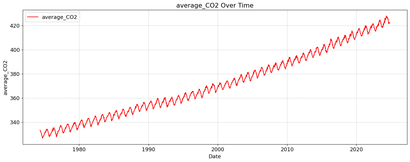
The quantity of CO2 is determined and described by the chemical term “mole fraction”, defined as the number of carbon dioxide molecules in a given number of molecules of air, after removal of water vapor. For example, 413 parts per million of CO2 (abbreviated as ppm) means that in every million molecules of (dry) air there are on average 413 CO2 molecules.

1 Importing libraries

import pandas as pd
import numpy as np
import matplotlib.pyplot as plt
import seaborn as sns
from scipy.stats import kendalltau
from helpers import (coerce_into_full_datetime, add_missing_one_year_rows, 
                      plot_column, add_missing_dates, plot_rolling_correlations, 
                      interpret_p_value, plot_lagged_correlations, plot_entire_df)
from statsmodels.tsa.stattools import adfuller, grangercausalitytests
import warnings
warnings.filterwarnings('ignore')

2 Importation, checks and formatting of station data

df_station = pd.read_csv('data_project - Sheet1.csv')
df_station

	year	month	day	decimal	average	ndays	1 year ago	10 years ago	increase since 1800
0	year	5	19	1974.3795	333.37	5	-999.99	-999.99	50.40
1	year	5	26	1974.3986	332.95	6	-999.99	-999.99	50.06
2	year	6	2	1974.4178	332.35	5	-999.99	-999.99	49.60
3	year	6	9	1974.4370	332.20	7	-999.99	-999.99	49.65
4	year	6	16	1974.4562	332.37	7	-999.99	-999.99	50.06
...	...	...	...	...	...	...	...	...	...
2626	2024	9	15	2024.7063	421.98	7	418.33	395.24	145.49
2627	2024	9	22	2024.7254	421.71	2	418.28	395.47	145.32
2628	2024	9	29	2024.7445	421.95	4	418.35	395.61	145.56
2629	2024	10	6	2024.7637	422.16	4	418.47	395.73	145.68
2630	2024	10	13	2024.7828	422.62	5	419.56	395.86	145.97

2631 rows × 9 columns

invalid_10years = (df_station['10 years ago'] == -999.99).sum()
invalid_10years

np.int64(540)

We can use the information from the other columns to create a valid datetime format.

The ‘decimal’ column along with the ‘day’ and ‘month’ columns can be used to adjust the datetime index accordingly

df_station['year'] = df_station['year'].astype(str).str.strip()
mask = df_station['year'] == 'year'
df_station.loc[mask, 'year'] = df_station.loc[mask, 'decimal'].fillna(0).apply(lambda x: int(float(x)))

df_station.drop(columns = ['decimal'], inplace = True)
df_station = coerce_into_full_datetime(df_station)

invalid_average = (df_station['average'] == -999.99).sum()
invalid_1year = (df_station['1 year ago'] == -999.99).sum()
invalid_10years = (df_station['10 years ago'] == -999.99).sum()

print(invalid_average)
print(invalid_1year)
print(invalid_10years)

18
70
540

We are using the data from the ‘1 year ago’ and ‘10 years ago’ columns to include and adjust missing datetimes, thus giving us a richer dataframe which would allow us to capture the trend effectively.

df_station = add_missing_dates(df_station) # using the function to create new rows using the '10 year ago' column
df_station = add_missing_one_year_rows(df_station) # using the function to create new rows using the '1 year ago' column
df_station.drop(df_station[df_station['average'] == -999.99].index, inplace=True)

3 Importation, preprocessing and evaluation of feature importance from Open Meteo weather data

df_history = pd.read_csv(r'open-meteo-19.44N155.62E0m - Sheet1.csv', skiprows=3)
df_history.index = pd.to_datetime(df_history.index).strftime('%Y-%m-%d %H:%M:%S')
df_history.reset_index(inplace=True)
df_history.set_index('time', inplace=True)
df_history.drop(columns = 'index', inplace = True)
df_history.index = pd.to_datetime(df_history.index)
df_history = df_history.resample('D').mean()

# Creating df on dates when station data and Open Meteo data overlap

common_dates = df_history.index.intersection(df_station.index)
df_history = df_history.loc[common_dates]

df_history

	temperature_2m (°C)	relative_humidity_2m (%)	dew_point_2m (°C)	precipitation (mm)	pressure_msl (hPa)	surface_pressure (hPa)	et0_fao_evapotranspiration (mm)	wind_speed_10m (m/s)	soil_temperature_0_to_7cm (°C)
1974-05-19	25.341667	70.666667	19.587500	0.091667	1009.866667	1009.866667	0.194583	7.951667	27.300000
1974-05-25	26.820833	83.041667	23.716667	0.004167	1014.900000	1014.900000	0.213750	5.412083	27.833333
1974-05-26	26.445833	81.000000	22.929167	0.012500	1014.766667	1014.766667	0.220833	6.092083	27.666667
1974-06-01	26.587500	81.416667	23.120833	0.025000	1012.683333	1012.683333	0.217500	4.369167	28.033333
1974-06-02	26.600000	80.833333	23.037500	0.029167	1011.666667	1011.666667	0.208333	3.939167	28.166667
...	...	...	...	...	...	...	...	...	...
2024-09-15	28.470833	76.041667	23.812500	0.425000	1009.612500	1009.612500	0.215417	7.975000	29.450000
2024-09-22	28.937500	76.416667	24.341667	0.045833	1013.208333	1013.208333	0.235833	7.489167	29.591667
2024-09-29	28.983333	75.750000	24.245833	0.004167	1013.491667	1013.491667	0.232083	6.991667	29.691667
2024-10-06	28.591667	76.458333	24.045833	0.095833	1012.320833	1012.320833	0.207917	5.662083	29.608333
2024-10-13	27.341667	83.375000	24.279167	0.437500	1010.179167	1010.179167	0.152500	6.735000	29.416667

5174 rows × 9 columns

df_station_column = df_station[['average']]
df_CO2_meteo = df_history.join(df_station_column, how='inner')

3.1 Evaluating correlations between weather data and CO2 levels from station data

# Computing Kendall's Tau correlation matrix

kendall_corr = df_CO2_meteo.corr(method='kendall')

plt.figure(figsize=(12, 6))
sns.heatmap(kendall_corr, annot=True, cmap='coolwarm', fmt=".2f")
div_palette = sns.color_palette("RdBu", 12)
plt.rcParams.update({'font.size': 13})
plt.title("Kendall Correlation Heatmap")
plt.show()

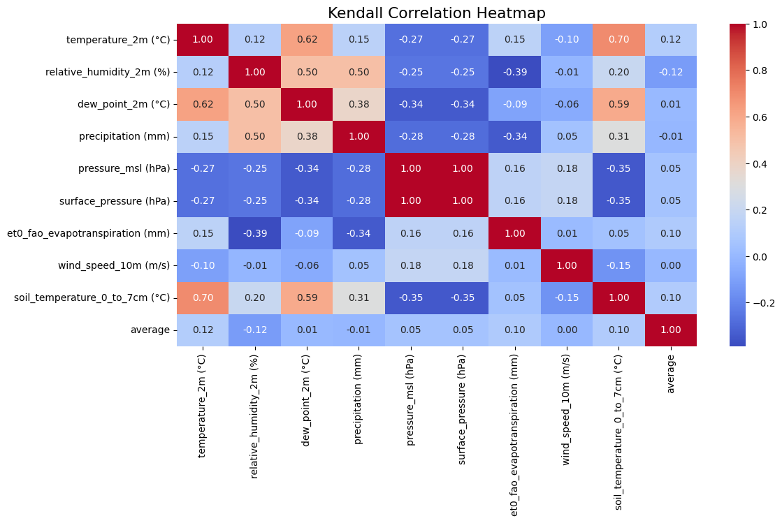
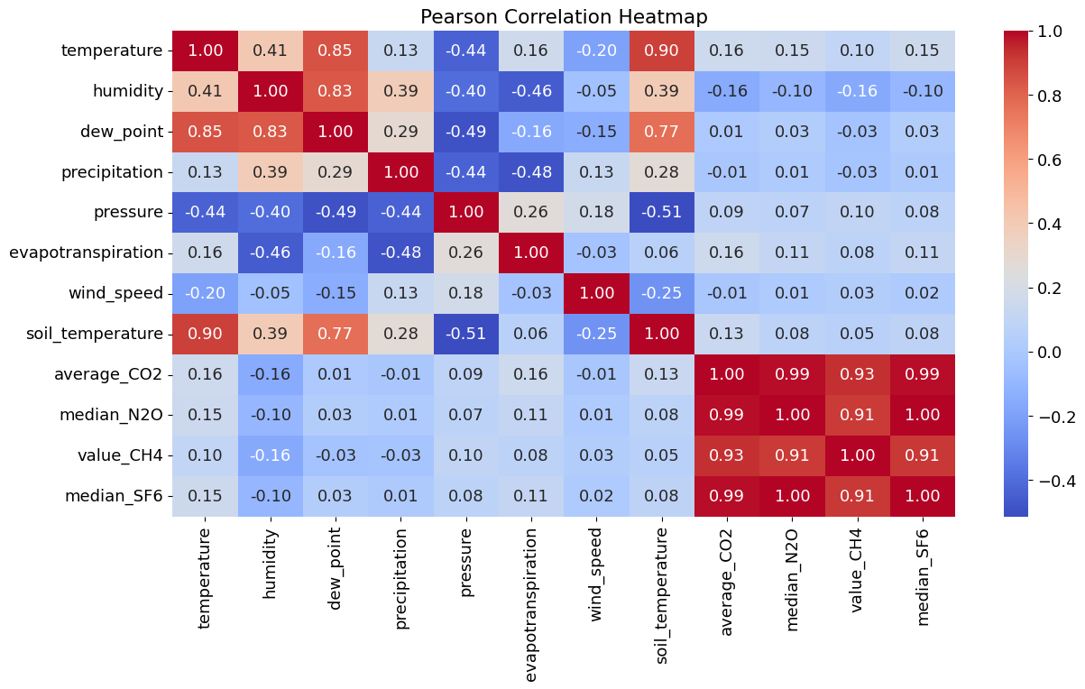
Surprisingly and unfortunately, there seems to be little to no correlation between the weather data and the average levels of CO2 at this particular location.

However further testing and assessment is needed before drawing final conclusions.

df_CO2_meteo.drop(['surface_pressure (hPa)'],axis=1,inplace = True)

df_CO2_meteo.rename(columns={'average': 'average_CO2', 'temperature_2m (°C)' : 'temperature', 
                             'relative_humidity_2m (%)':'humidity', 'dew_point_2m (°C)' : 'dew_point',
                             'precipitation (mm)' : 'precipitation', 'pressure_msl (hPa)' : 'pressure',
                             'et0_fao_evapotranspiration (mm)' : 'evapotranspiration', 
                             'wind_speed_10m (m/s)' : 'wind_speed', 'soil_temperature_0_to_7cm (°C)' : 'soil_temperature'}, inplace=True)

df_CO2_meteo.to_csv('df_CO2_meteo.csv', index=True)

4 N2O Importation and analysis

df_N2O = pd.read_csv(r'mlo_N2O_Day.csv', skiprows = 1)

new_column_names = ['year', 'month', 'day', 'median_N2O', 'std._dev.N2O', 'samplesN20']
df_N2O.columns = new_column_names
df_N2O

	year	month	day	median_N2O	std._dev.N2O	samplesN20
0	1998	11	28	NaN	NaN	0
1	1998	11	29	NaN	NaN	0
2	1998	11	30	NaN	NaN	0
3	1998	12	1	NaN	NaN	0
4	1998	12	2	NaN	NaN	0
...	...	...	...	...	...	...
8760	2022	11	23	337.97	1.08	24
8761	2022	11	24	337.61	0.98	24
8762	2022	11	25	337.51	1.02	23
8763	2022	11	26	337.02	0.96	23
8764	2022	11	27	337.51	0.94	24

8765 rows × 6 columns

df_N2O = coerce_into_full_datetime(df_N2O) # using the `year`, `month` and `day` columns

	median_N2O	std._dev.N2O	samplesN20
datetime
1998-11-28	NaN	NaN	0
1998-11-29	NaN	NaN	0
1998-11-30	NaN	NaN	0
1998-12-01	NaN	NaN	0
1998-12-02	NaN	NaN	0
...	...	...	...
2022-11-23	337.97	1.08	24
2022-11-24	337.61	0.98	24
2022-11-25	337.51	1.02	23
2022-11-26	337.02	0.96	23
2022-11-27	337.51	0.94	24

8765 rows × 3 columns

df_N2O.interpolate(method='time', inplace=True)
df_N2O.fillna(method='ffill', inplace=True)
df_N2O.fillna(method='bfill', inplace=True)

df_N2O

	median_N2O	std._dev.N2O	samplesN20
datetime
1998-11-28	315.59	0.38	0
1998-11-29	315.59	0.38	0
1998-11-30	315.59	0.38	0
1998-12-01	315.59	0.38	0
1998-12-02	315.59	0.38	0
...	...	...	...
2022-11-23	337.97	1.08	24
2022-11-24	337.61	0.98	24
2022-11-25	337.51	1.02	23
2022-11-26	337.02	0.96	23
2022-11-27	337.51	0.94	24

8765 rows × 3 columns

5 Methane importation and analysis

df_CH4 = pd.read_csv(r'mlo_CH4_Day.csv')

new_column_names = [
    "site_code", "year", "month", "day", "hour", "minute", "second",
    "datetime", "time_decimal", "midpoint_time", "value_CH4", "value_std_dev_CH4",
    "nvalue_CH4", "latitude", "longitude", "altitude", "elevation", "intake_height", "qcflag"
]

df_CH4.columns = new_column_names

df_CH4.drop(
    columns=["site_code", "year", "month", "day", "hour", "minute", "second", "time_decimal",
             "midpoint_time", "latitude", "longitude", "altitude", "elevation", "intake_height", "qcflag"],
    inplace=True
)
df_CH4["datetime"] = pd.to_datetime(df_CH4["datetime"]).dt.date
df_CH4.set_index("datetime", inplace=True)

df_CH4

	value_CH4	value_std_dev_CH4	nvalue_CH4
datetime
1987-01-02	-999.99	-99.99	0
1987-01-03	-999.99	-99.99	0
1987-01-04	-999.99	-99.99	0
1987-01-05	-999.99	-99.99	0
1987-01-06	-999.99	-99.99	0
...	...	...	...
2024-04-26	1977.78	0.85	7
2024-04-27	1969.78	2.95	7
2024-04-28	1955.87	7.38	7
2024-04-29	1924.00	0.84	7
2024-04-30	1924.86	0.50	7

13634 rows × 3 columns

invalid_CH4 = (df_CH4['value_CH4'] == -999.99).sum()
invalid_CH4

np.int64(906)

Since the invalid rows in this dataset are of a miniscule amount in comparison to the size of the whole data, completely removing them does no harm.

df_CH4 = df_CH4.loc[df_CH4["value_CH4"] != -999.99]

6 SF6 importation and checks

df_SF6 = pd.read_csv(r'mlo_SF6_Day.csv', skiprows = 1)

new_column_names = ['year', 'month', 'day', 'median_SF6', 'std.dev_SF6', 'samples']
df_SF6.columns = new_column_names

df_SF6['year'] = df_SF6['year'].astype(str).str.strip()
mask = df_SF6['year'] == 'year'

df_SF6 = coerce_into_full_datetime(df_SF6) # using the `year`, `month` and `day` columns
df_SF6

	median_SF6	std.dev_SF6	samples
datetime
1998-11-29	NaN	NaN	0
1998-11-30	NaN	NaN	0
1998-12-01	NaN	NaN	0
1998-12-02	NaN	NaN	0
1998-12-03	NaN	NaN	0
...	...	...	...
2022-11-23	11.594	0.052	24
2022-11-24	11.518	0.049	24
2022-11-25	11.455	0.047	24
2022-11-26	11.394	0.045	24
2022-11-27	11.405	0.046	24

8764 rows × 3 columns

df_SF6.interpolate(method='time', inplace=True)
df_SF6.fillna(method='ffill', inplace=True)
df_SF6.fillna(method='bfill', inplace=True)

7 Merging and visualising all data

df_CO2_meteo.rename_axis('datetime', inplace=True)

plot_column(df_CO2_meteo, 'average_CO2', 'red')
plot_column(df_N2O, 'median_N2O', 'blue')
plot_column(df_CH4, 'value_CH4', 'green')
plot_column(df_SF6, 'median_SF6', 'magenta')
plt.tight_layout

dfs = [df.copy() for df in [df_CO2_meteo, df_N2O, df_CH4, df_SF6]]
for i in range(len(dfs)):
    dfs[i].index = pd.to_datetime(dfs[i].index)  # Converting index to proper datetime64[ns]

start_date = df_CO2_meteo.index.min()  # Get the earliest date from df_CO2_meteo
dfs = [df[df.index >= start_date] for df in dfs]

df_combined_outer = pd.concat(
    [dfs[0][['temperature', 'humidity', 'dew_point', 'precipitation', 'pressure',
             'evapotranspiration', 'wind_speed', 'soil_temperature', 'average_CO2']],
     dfs[1][["median_N2O"]],
     dfs[2][["value_CH4"]],
     dfs[3][["median_SF6"]]],
    axis=1, join="outer")

dfs = [df.copy() for df in [df_CO2_meteo, df_N2O, df_CH4, df_SF6]]
for i in range(len(dfs)):
    dfs[i].index = pd.to_datetime(dfs[i].index)  # Converting index to proper datetime64[ns]

start_date = df_CO2_meteo.index.min()  # Get the earliest date from df_CO2_meteo
dfs = [df[df.index >= start_date] for df in dfs]

df_combined_inner = pd.concat(
    [dfs[0][['temperature', 'humidity', 'dew_point', 'precipitation', 'pressure',
             'evapotranspiration', 'wind_speed', 'soil_temperature', 'average_CO2']],
     dfs[1][["median_N2O"]],
     dfs[2][["value_CH4"]],
     dfs[3][["median_SF6"]]],
    axis=1, join="inner")

columns_to_fill = ['temperature', 'humidity', 'dew_point', 'precipitation', 'pressure',
                   'evapotranspiration', 'wind_speed', 'soil_temperature', 'average_CO2']

df_combined_outer[columns_to_fill] = df_combined_outer[columns_to_fill].interpolate(method='time')
df_combined_outer[columns_to_fill] = df_combined_outer[columns_to_fill].fillna(method='ffill') # Forward fill remaining missing values
df_combined_outer[columns_to_fill] = df_combined_outer[columns_to_fill].fillna(method='bfill') # Backward fill remaining missing values

plot_entire_df(df_combined_outer)

8 Visualising Correlations

# Computing Kendall's Tau correlation matrix

kendall_corr = df_combined_outer.corr(method='kendall')

plt.figure(figsize=(14, 7))
sns.heatmap(kendall_corr, annot=True, cmap='coolwarm', fmt=".2f")
plt.title("Kendall Correlation Heatmap")
plt.show()

# Compute Pearson's Tau correlation matrix
pearson_corr = df_combined_outer.corr(method='pearson')

plt.figure(figsize=(14, 7))
sns.heatmap(pearson_corr, annot=True, cmap='coolwarm', fmt=".2f")
plt.title("Pearson Correlation Heatmap")
plt.show()

Pearson’s correlation measures the linear relationship between variables.

The correlation coefficient ranges from -1 to +1, where -1 indicates a perfect negative linear relationship, +1 indicates a perfect positive linear relationship, and 0 indicates no linear relationship.

However, it has a limitation: it only captures linear relationships and can miss other types of relationships between variables.

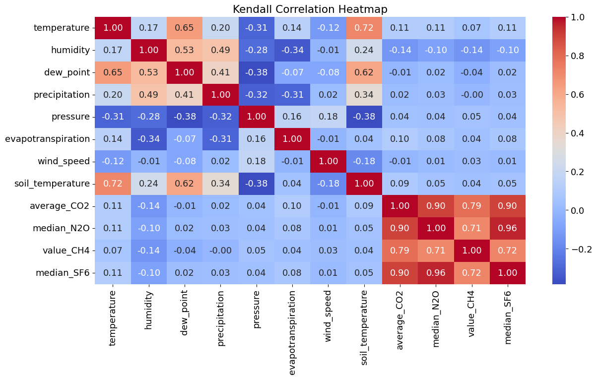
Kendall’s Tau takes a different approach. Instead of measuring linear relationships, it looks at the concordance between variables - essentially, whether they tend to move in the same direction. It’s measuring the tendency of the variables to increase or decrease together, without assuming anything about the shape of that relationship.

In the context of environmental data like CO2 levels, temperature, and other climate variables, Kendall’s Tau might be particularly useful because environmental relationships aren’t always linear, and the data often contains outliers or follows non-normal distributions.

plot_rolling_correlations(df_combined_inner)

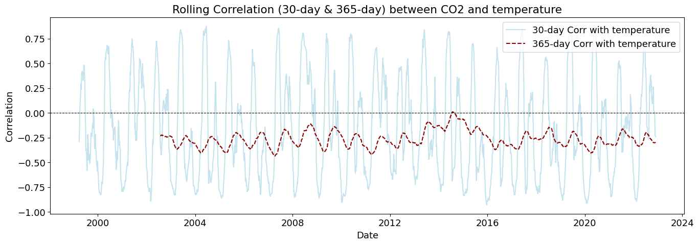
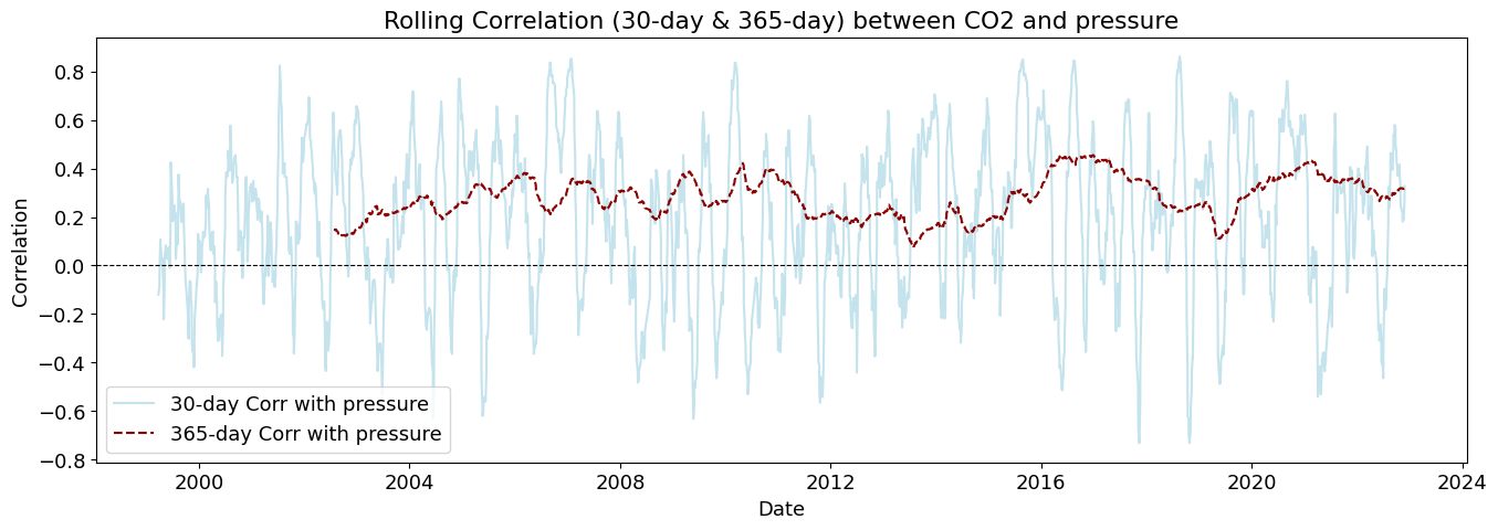
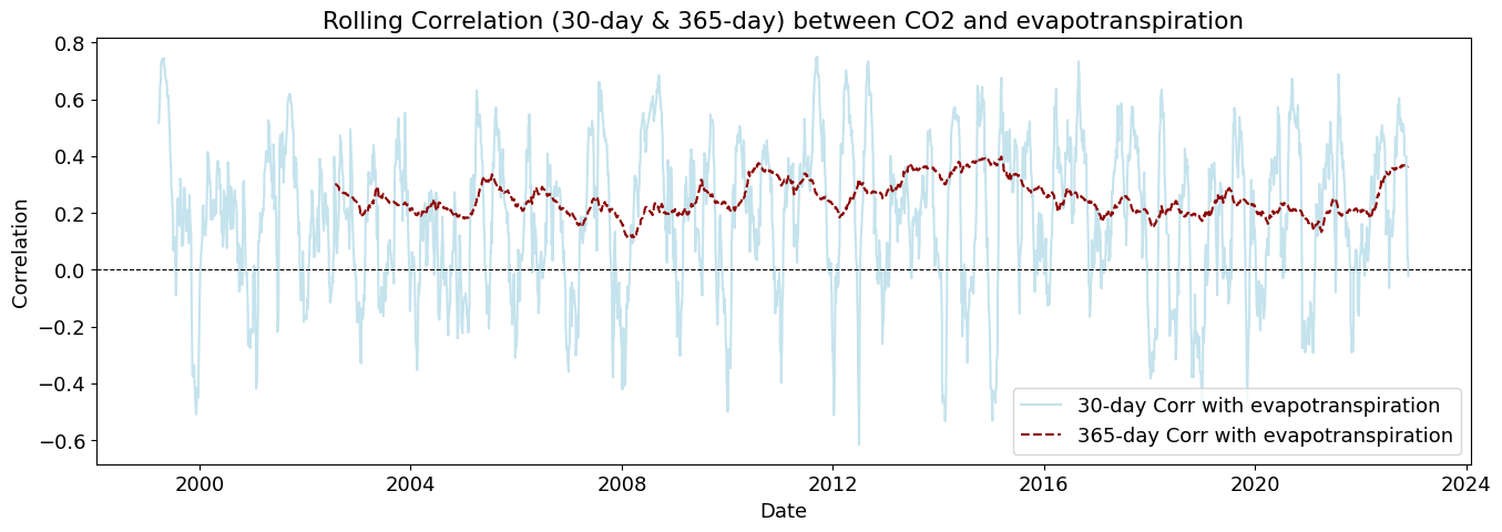
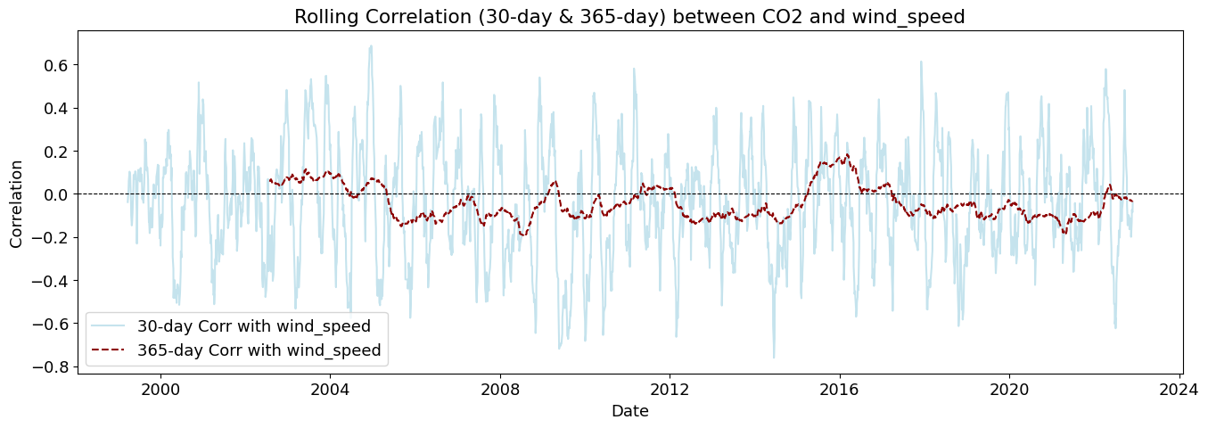
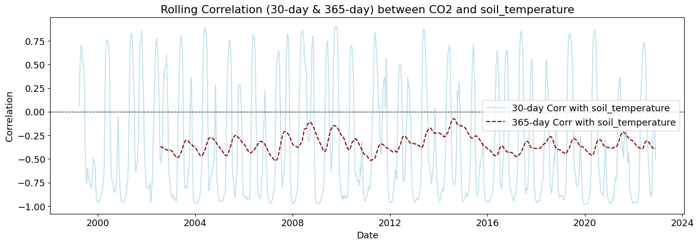
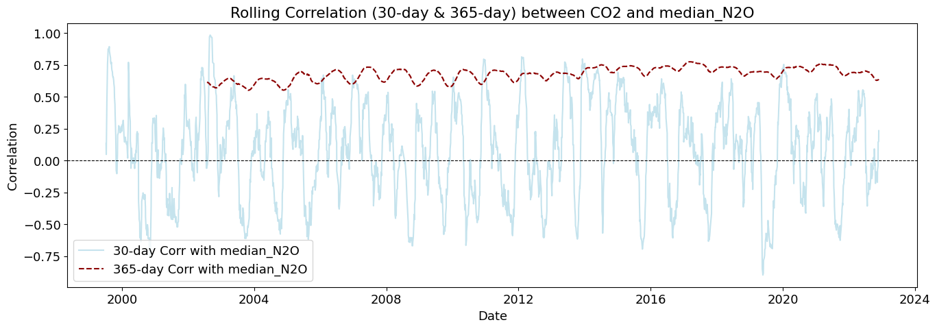
Rolling correlations (also called moving correlations) are a dynamic way to measure how the relationship between two variables changes over time. Unlike a single correlation coefficient that shows one number for an entire dataset, rolling correlations show how the correlation evolves throughout a time series.

Rolling correlations can be used in environmental studies to understand how relationships between variables shift with seasonal or long-term changes.

# Checking for stationarity (Augmented Dickey-Fuller Test)
def check_stationarity(series, variable_name):
    result = adfuller(series.dropna())
    p_value = result[1]
    return p_value

stationarity_results = {col: check_stationarity(df_combined_inner[col], col) for col in df_combined_inner.columns}

max_lag = 12
granger_results = {}

# Performing Granger Causality tests
for col in df_combined_inner.columns:
    if col != "average_CO2":
        test_result = grangercausalitytests(df_combined_inner[['average_CO2', col]].dropna(), max_lag, verbose=False)
        granger_results[col] = {lag: test_result[lag][0]['ssr_ftest'][1] for lag in range(1, max_lag + 1)}

stationarity_results

{'temperature': np.float64(9.451145188179234e-22),
 'humidity': np.float64(1.2067943715819874e-12),
 'dew_point': np.float64(1.2150381839441513e-19),
 'precipitation': np.float64(7.824982759354124e-20),
 'pressure': np.float64(6.824231580012553e-12),
 'evapotranspiration': np.float64(5.673478319719433e-14),
 'wind_speed': np.float64(8.298941795111292e-30),
 'soil_temperature': np.float64(1.6253595748496084e-23),
 'average_CO2': np.float64(0.8630583937959493),
 'median_N2O': np.float64(0.999004879583799),
 'value_CH4': np.float64(0.6729054440779778),
 'median_SF6': 1.0}

The ADF test checks whether a time series data is stationary, which is crucial for many statistical analyses. A stationary time series has consistent statistical properties over time - its mean and variance don’t change.

Granger Causality tests explore whether past values of one variable help predict future values of another. It’s testing the “statistical causality” - though it’s important to note that Granger causality doesn’t necessarily mean actual causation.

# Converting Granger causality test results into a readable dataFrame

granger_df = pd.DataFrame.from_dict(
    {var: [granger_results[var][lag] for lag in range(1, max_lag + 1)] for var in granger_results.keys()},
    orient='index',
    columns=[f'Lag {i}' for i in range(1, max_lag + 1)]
)

granger_df["Interpretation"] = granger_df.apply(lambda row: interpret_p_value(row.values), axis=1)
granger_df

	Lag 1	Lag 2	Lag 3	Lag 4	Lag 5	Lag 6	Lag 7	Lag 8	Lag 9	Lag 10	Lag 11	Lag 12	Interpretation
temperature	7.720947e-25	5.497089e-21	7.705556e-26	9.829507e-24	7.675065e-19	3.120083e-17	8.219184e-13	2.203910e-12	5.638884e-10	4.525774e-09	1.018310e-07	2.367689e-07	Strong causality (p < 0.01)
humidity	8.903531e-12	1.981891e-10	8.968556e-14	2.988373e-14	3.172161e-11	6.171779e-10	6.195866e-07	1.348078e-06	5.218207e-04	2.136951e-03	4.108305e-03	6.423288e-03	Strong causality (p < 0.01)
dew_point	8.067610e-25	4.458532e-21	8.264431e-26	3.584386e-24	1.393978e-19	4.411318e-18	1.616901e-13	7.524441e-13	4.799498e-09	3.827182e-08	1.586932e-07	3.114832e-07	Strong causality (p < 0.01)
precipitation	3.819164e-04	5.001872e-03	5.371408e-04	1.094697e-04	8.476688e-03	2.857322e-02	3.756680e-01	5.216954e-01	9.136631e-01	8.859372e-01	3.525676e-01	1.535244e-01	Moderate to low causality (p < 0.05 at some lags)
pressure	4.438619e-11	7.971067e-09	1.926409e-10	6.537783e-09	1.693316e-06	1.212028e-05	1.613346e-03	3.624291e-03	2.254627e-02	3.287454e-02	9.963901e-03	7.508465e-03	Moderate to low causality (p < 0.05 at some lags)
evapotranspiration	2.125455e-04	1.541215e-05	3.031203e-07	2.011486e-06	3.167283e-08	8.742475e-10	4.830566e-09	1.208496e-08	1.646039e-08	2.601857e-09	6.520648e-12	1.285255e-12	Strong causality (p < 0.01)
wind_speed	1.440207e-12	4.899939e-12	5.808182e-14	3.671966e-15	1.207507e-13	1.313350e-12	3.845556e-10	5.768298e-10	1.274597e-08	2.401023e-08	1.356298e-07	6.914299e-08	Strong causality (p < 0.01)
soil_temperature	4.069728e-32	1.903884e-26	1.176250e-39	1.926643e-37	1.831168e-32	1.178714e-30	7.919387e-24	3.344132e-23	6.174720e-22	7.789451e-21	5.191957e-22	2.197068e-21	Strong causality (p < 0.01)
median_N2O	8.008445e-05	4.118513e-05	8.078303e-04	6.303455e-04	1.439309e-04	3.025065e-06	1.612906e-08	1.365409e-08	6.937741e-13	4.135353e-14	9.966893e-18	1.458885e-18	Strong causality (p < 0.01)
value_CH4	6.094348e-06	1.821082e-13	1.783052e-19	2.951395e-22	2.037874e-23	3.249063e-25	1.223335e-22	4.499614e-22	6.773017e-15	8.673936e-14	5.394487e-13	1.508888e-12	Strong causality (p < 0.01)
median_SF6	8.433207e-04	2.402066e-07	7.523613e-06	7.130874e-08	2.532144e-11	1.648528e-12	6.471290e-15	7.232538e-15	5.658483e-17	3.503844e-18	1.710563e-20	1.563221e-22	Strong causality (p < 0.01)

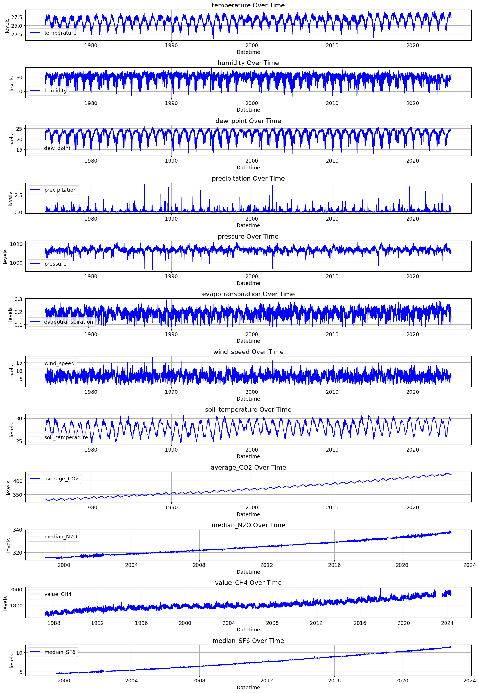
Results 1. Stationarity Check (Augmented Dickey-Fuller Test) CO₂ (average_C2O) is non-stationary → This means CO₂ has a trend and may need differencing to make it stationary before modeling. Although the meteorological data is mostly stationary, the gas related datasets (N₂O, CH₄, and SF₆) are non-stationary.

2. Granger Causality (p-values across 1-12 lags) Lower p-values (< 0.05) indicate strong causality. The smaller the p-value, the more significant the predictive relationship.

• Temperature (temperature_2m (°C)) ✅ Strong causality across all lags - Predicts future CO₂ trends
• Relative Humidity (relative_humidity_2m (%)) ✅ Significant up to lag 12 - Influences CO₂ levels, but weaker than temperature
• N₂O (median_N2O) ✅ Significant causality at longer lags - Has a delayed effect on CO₂
• CH₄ (value_CH4) ✅ Very strong causality - CH₄ changes predict CO₂ variations
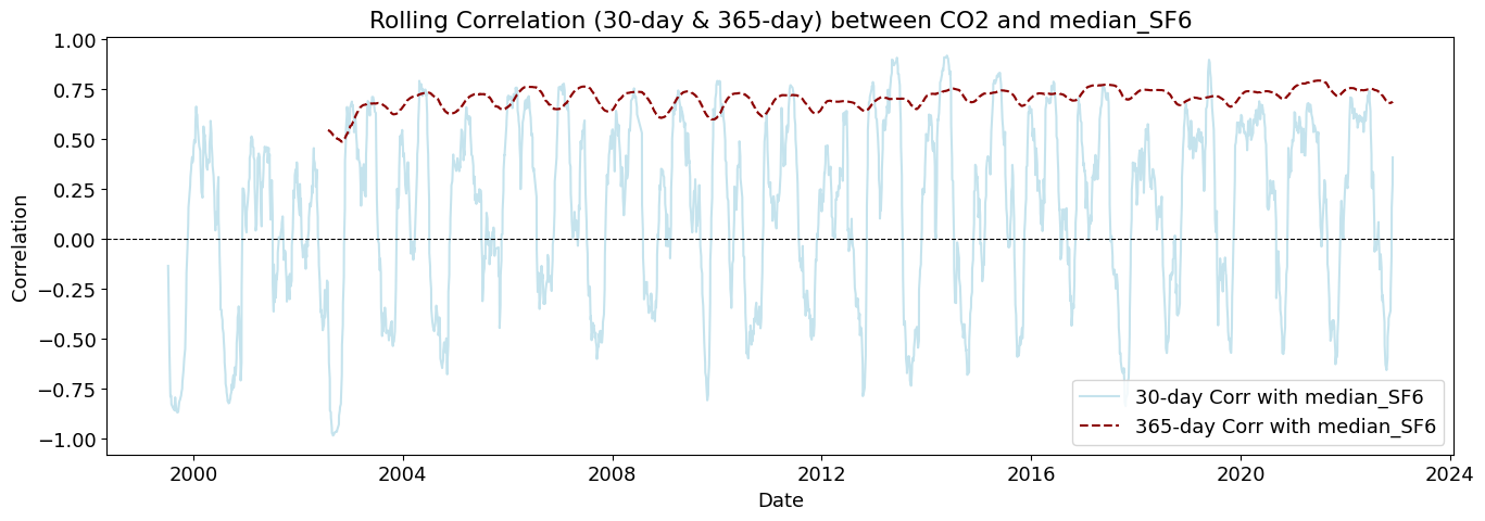
• SF₆ (median_SF6) ✅ Moderate causality at higher lags - SF₆ shows long-term predictive power

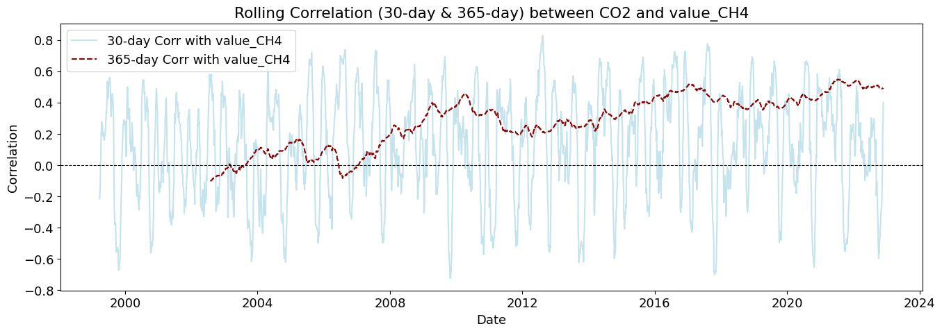
Temperature and CH₄ have a very strong causal effect and are the strongest predictor of CO₂

The p-values are extremely low, suggesting that past temperature values contain significant information about future CO₂ levels.

This makes sense since methane (CH₄) and CO₂ are both greenhouse gases affected by similar processes.

Humidity, N₂O, and SF₆ also predict CO₂, but to a lesser extent.

---

Why Did Pearson & Kendall Show Weak Correlation, But Granger Shows Strong Causality? The difference comes from how these methods analyze relationships.

1. Pearson/Kendall Correlation (Static, Instantaneous Relationship) These methods only measure direct relationships between variables at the same time. Pearson Correlation checks linear relationships at one point in time. Kendall Correlation looks at rank-based (monotonic) relationships but still without considering time delays. Since CO₂, temperature, and humidity might have delayed effects on each other, Pearson/Kendall may fail to detect a strong relationship.

2. Granger Causality (Temporal Dependency) This test considers past values of temperature, humidity, and other variables to see if they help predict future CO₂. Many climate and atmospheric processes do not act immediately—they take weeks or months to show an impact. Example: Higher temperatures today might increase plant respiration or ocean CO₂ release over the next few weeks or months. That’s why even if Pearson/Kendall showed weak relationships, Granger Causality detects delayed effects that standard correlation ignores.

Real-World Example of Delayed Causality in Climate Data

Temperature & CO₂: When temperatures rise, it may take weeks to months before we see a significant change in CO₂ levels due to ocean-atmosphere exchange. Humidity & CO₂: Humidity affects cloud cover, precipitation, and soil moisture, which influence carbon absorption and release but not immediately. Methane (CH₄) & CO₂: CH₄ breaks down into CO₂ over time, meaning its effects on CO₂ might appear after several months.

8.0.1 1 year in the past - analysis

plot_lagged_correlations(df_combined_inner, 'average_CO2', 365)

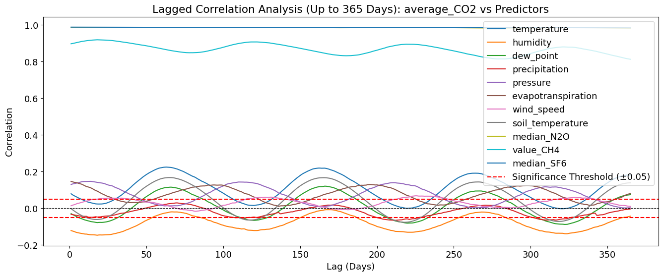
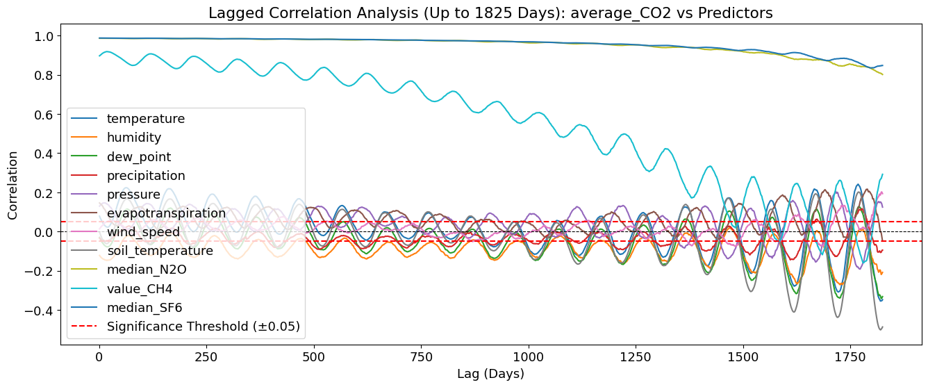
Key Observations: 🌡 Temperature (temperature_2m (°C)) shows a periodic pattern - The correlation peaks at around 90, 180, and 360 days. - This suggests a seasonal effect, where temperature changes predict CO₂ levels months later. - Possible explanation: Seasonal cycles of vegetation, ocean uptake, or industrial activity.

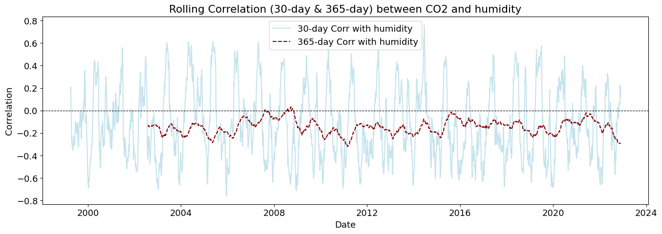
💧 Humidity (relative_humidity_2m (%)) has a weak but noticeable lag effect - Correlation is slightly negative, meaning higher humidity may be linked to lower CO₂ later. - This could be due to increased plant growth (photosynthesis) reducing CO₂.

🛑 N₂O (median_N2O) shows some delayed correlation

• N₂O is related to industrial activity and fossil fuel combustion.
• If N₂O increases, CO₂ might follow due to shared emission sources.

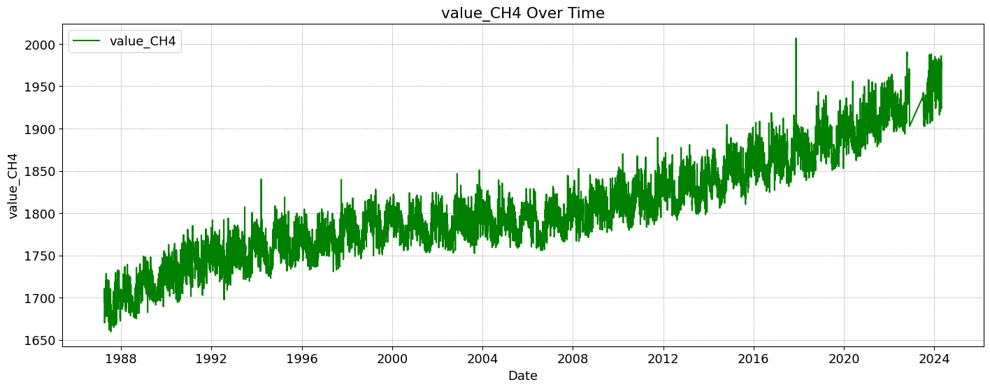
*🔥 Methane (value_CH4) has a strong positive correlation with CO₂ over time

• CH₄ and CO₂ both contribute to greenhouse effects.
• CH₄ breaks down into CO₂ over time, explaining why higher CH₄ leads to increased CO₂ later.

🌎 SF₆ (median_SF6) shows the strongest overall correlation

• SF₆ is a long-lived greenhouse gas, and its correlation with CO₂ is almost constant. This suggests shared sources or long-term emission trends.

🔬 Interpretation - Temperature and CH₄ are the strongest predictors of CO₂ over time. - The delayed effects (~90 to 360 days) explain why Pearson/Kendall correlation missed these relationships. - There is a clear seasonal component, especially for temperature and humidity. - Industrial gases (N₂O, SF₆) show long-term trends in relation to CO₂.

8.0.2 5 year in the past - analysis

plot_lagged_correlations(df_combined_inner, 'average_CO2', 1825)

📉 Temperature (temperature_2m (°C)) shows Strong Multi-Year Cycles - Clear periodic pattern every ~365 days → Suggests annual climate cycles affecting CO₂. - Peaks every ~1 year, aligning with seasonal and yearly CO₂ fluctuations.

💧 Humidity (relative_humidity_2m (%)) Shows Opposite Cycles - Correlation oscillates inversely to temperature. - Suggests that higher humidity is associated with lower future CO₂ levels, likely linked to vegetation absorption and precipitation cycles.

🔥 CH₄ (value_CH4) and SF₆ (median_SF6) Show Strong Long-Term Correlations - they maintain high correlation for multiple years.

📈 N₂O (median_N2O) Shows Long-Term Influence - it maintains a high correlation for several years.

The yearly cycles suggest that seasonality must be considered in CO₂ forecasting models.

8.0.3 10 year back analysis

plot_lagged_correlations(df_combined_inner, 'average_CO2', 3650)

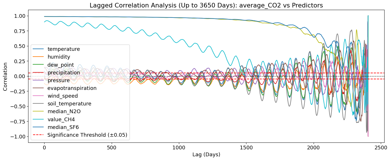
🔍 Very Long-Term Lagged Correlation Analysis (10 Years)

This plot extends the lagged correlation window to 10 years (3650 days) to examine even longer-term dependencies between CO₂ and its predictors.

🌡 Temperature (temperature_2m (°C)) Shows a Strong Multi-Year Cycle

• Clear oscillations approximately every year (365 days) - suggests strong seasonal and multi-year trends in CO₂.

💧 Humidity (relative_humidity_2m (%)) - shows an inverse correlation to temperature. - Indicates that higher humidity leads to lower CO₂ after several months/years (likely due to enhanced vegetation growth, precipitation, and CO₂ absorption).

🔥 N₂O (median_N2O) and SF₆ (median_SF6) Maintain Strong Long-Term Correlations

• They consistently correlate with CO₂ across multiple years - suggests shared emission sources or slow accumulation effects over time.

📈 CH₄ (value_CH4) Shows a Gradual Decrease in Correlation Over Time

• The influence on CO₂ appears strongest in the first few years but then declines.

📉 After ~8-10 Years, Correlations Become More Unstable

Around 2500-3500 days (7-10 years), the correlations become noisier. This could be due to external climate variability, policy changes, or model limitations in capturing such long-term effects.

🌍 Implications for Long-Term CO₂ Forecasting - Annual cycles are clearly visible, meaning that any CO₂ forecasting model should incorporate seasonality. - Humidity has a delayed inverse effect, possibly due to its influence on carbon sinks. - Industrial pollutants show shorter-term influence, making them more useful for mid-term (1-5 year) forecasting.

df_combined_inner.drop(columns = ['precipitation', 'wind_speed', 'dew_point', 'pressure'])
df_combined_outer.drop(columns = ['precipitation', 'wind_speed', 'dew_point', 'pressure'])
df_full_CO2 = df_combined_outer[['average_CO2']]

df_combined_inner.to_csv('df_combined_inner.csv', index=True)
df_combined_outer.to_csv('df_combined_outer.csv', index=True)
df_full_CO2.to_csv('df_full_CO2.csv', index=True)